Kernel density estimation: Difference between revisions
CSV import |
CSV import |
||
| Line 38: | Line 38: | ||
{{Statistics-stub}} | {{Statistics-stub}} | ||
== Kernel_density_estimation == | |||
<gallery> | |||
File:Kernel_density.svg|Kernel density plot | |||
File:Comparison_of_1D_histogram_and_KDE.png|Comparison of 1D histogram and KDE | |||
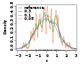
File:Comparison_of_1D_bandwidth_selectors.png|Comparison of 1D bandwidth selectors | |||
File:Kernel_density_estimation,_comparison_between_rule_of_thumb_and_solve-the-equation_bandwidth.png|Kernel density estimation, comparison between rule of thumb and solve-the-equation bandwidth | |||
</gallery> | |||
Latest revision as of 04:36, 18 February 2025
Kernel Density Estimation (KDE) is a non-parametric way to estimate the probability density function of a random variable. KDE is a fundamental data smoothing problem where inferences about the population are made, based on a finite data sample. It is used in various fields such as signal processing, data mining, and machine learning to analyze and visualize the underlying distribution of data.
Overview[edit]
Kernel density estimation is a method to estimate the probability density function (PDF) of a continuous random variable. It is used when the shape of the distribution is unknown, and it aims to provide a smooth estimate based on a finite sample. The KDE is a sum of kernels, usually symmetric and unimodal, which are centered at the sample points. The most common choice of kernel is the Gaussian kernel, but other kernels like Epanechnikov, Tophat, and Exponential can be used depending on the application.
Mathematical Formulation[edit]
Given a set of n independent and identically distributed samples X = {x_1, x_2, ..., x_n} from some distribution with an unknown density f, the kernel density estimator f̂ is defined as:
\[ f̂(x) = \frac{1}{nh} \sum_{i=1}^{n} K\left(\frac{x - x_i}{h}\right) \]
where K is the kernel — a non-negative function that integrates to one and has mean zero — and h is a smoothing parameter called the bandwidth. The choice of h is critical as it controls the trade-off between bias and variance in the estimate. Too small a bandwidth leads to a very bumpy density estimate (overfitting), while too large a bandwidth oversmooths the density estimate (underfitting).
Bandwidth Selection[edit]
The selection of the bandwidth h is crucial in KDE and can significantly affect the estimator's performance. Several methods for selecting the optimal bandwidth exist, including the rule of thumb, cross-validation, and plug-in approaches. The rule of thumb is simple but may not be optimal for data that is not normally distributed. Cross-validation methods, such as least squares cross-validation, aim to minimize the difference between the estimated and the true density functions. Plug-in methods provide a more automated approach to bandwidth selection but require assumptions about the underlying density.
Applications[edit]
Kernel density estimation is widely used in various fields for data analysis and visualization:
- In Economics, KDE is used to analyze income distributions and financial market data.
- In Environmental Science, it helps in modeling the distribution of species and pollution levels.
- In Machine Learning and Data Mining, KDE is employed for density estimation, clustering, and anomaly detection.
- In Signal Processing, it is used for noise reduction and signal reconstruction.
Advantages and Limitations[edit]
The main advantage of KDE is its flexibility in modeling distributions without assuming a specific parametric form. However, KDE has limitations, including sensitivity to bandwidth selection and computational complexity with large datasets. Additionally, KDE may perform poorly with multi-modal distributions or when the data has significant outliers.
See Also[edit]
References[edit]
<references/>

This article is a statistics-related stub. You can help WikiMD by expanding it!
Kernel_density_estimation[edit]
-
 Kernel density plot
 -
 Comparison of 1D histogram and KDE
 -
 Comparison of 1D bandwidth selectors
 -
 Kernel density estimation, comparison between rule of thumb and solve-the-equation bandwidth


