Ornstein–Uhlenbeck process: Difference between revisions
CSV import |
CSV import |
||
| Line 48: | Line 48: | ||
[[Category:Financial mathematics]] | [[Category:Financial mathematics]] | ||
{{math-stub}} | {{math-stub}} | ||
<gallery> | |||
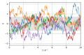
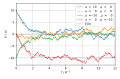
File:Ornstein-Uhlenbeck-5traces.svg|Ornstein–Uhlenbeck process | |||
File:OrnsteinUhlenbeckProcess3D.svg|Ornstein–Uhlenbeck process | |||
File:Leonard_Ornstein_mural,_Oosterkade,_Utrecht,_2021_-_1_(cropped)_-_Ornstein's_1930_random_walk_formula.jpg|Leonard Ornstein mural, Oosterkade, Utrecht, 2021 | |||
File:Leonard_Ornstein_mural,_Oosterkade,_Utrecht,_2021_-_1.jpg|Leonard Ornstein mural, Oosterkade, Utrecht, 2021 | |||
File:Ornstein-Uhlenbeck-traces-a-mu.svg|Ornstein–Uhlenbeck process | |||
</gallery> | |||
Latest revision as of 11:32, 18 February 2025
Ornstein–Uhlenbeck process is a type of stochastic process that describes the velocity of a massive Brownian particle under the influence of friction. It is named after Leonard Ornstein and George Eugene Uhlenbeck. The process is a stationary Gauss-Markov process, making it a continuous-time analog of the discrete-time autoregressive process of order 1, or AR(1) process. It is a solution to the Langevin equation with a linear restoring force and Gaussian white noise, representing a model for the velocity of a particle in a fluid undergoing Brownian motion.
Definition[edit]
The Ornstein–Uhlenbeck process \(U(t)\) can be defined as the solution to the stochastic differential equation (SDE):
\[dU(t) = \theta (\mu - U(t))dt + \sigma dW(t)\]
where:
- \( \theta > 0 \) is the rate of mean reversion,
- \( \mu \) is the long-term mean level,
- \( \sigma > 0 \) is the volatility,
- \( W(t) \) is a Wiener process, and
- \( t \) represents time.
Properties[edit]
The Ornstein–Uhlenbeck process exhibits several key properties:
- It is mean-reverting, meaning it tends to drift towards its long-term mean \( \mu \) over time.
- It is a stationary process, implying that its statistical properties do not change over time.
- It is a Markov process, indicating that future values of the process depend only on the current state, not on the path taken to arrive at that state.
- It has Gaussian increments, which means that the changes in the process over any two points in time are normally distributed.
Applications[edit]
The Ornstein–Uhlenbeck process has wide applications across various fields:
- In finance, it is used to model interest rates, currency exchange rates, and commodity prices.
- In physics, it models the velocity of a particle in a fluid.
- In biology, it can describe the fluctuation in populations or the spread of viruses.
- In engineering, it is applied in signal processing and control systems.
Mathematical Solution[edit]
The exact solution of the Ornstein–Uhlenbeck SDE is given by:
\[U(t) = U(0)e^{-\theta t} + \mu(1 - e^{-\theta t}) + \sigma \int_0^t e^{-\theta (t-s)} dW(s)\]
This solution shows how the process evolves over time from an initial state \(U(0)\).
See Also[edit]
References[edit]
<references/>

This article is a mathematics-related stub. You can help WikiMD by expanding it!
-
 Ornstein–Uhlenbeck process
 -
 Ornstein–Uhlenbeck process
 -
 Leonard Ornstein mural, Oosterkade, Utrecht, 2021
 -
 Leonard Ornstein mural, Oosterkade, Utrecht, 2021
 -
 Ornstein–Uhlenbeck process


