Lagrange multiplier

Lagrange Multipliers are a strategy used in calculus for finding the local maxima and minima of a function subject to equality constraints. This method is named after the Italian-French mathematician Joseph-Louis Lagrange. It is a powerful tool in optimization, especially in the fields of economics, engineering, and physics, where it is often necessary to optimize a function under certain conditions.

Overview

The basic idea behind Lagrange multipliers is to transform a constrained optimization problem into an unconstrained optimization problem. This is achieved by introducing an auxiliary variable, known as the Lagrange multiplier, for each constraint. The method involves setting up a new function, called the Lagrangian, which incorporates the original function to be optimized and the constraints, each multiplied by their corresponding Lagrange multiplier.

Mathematical Formulation

Consider a function \(f(x, y)\) that we wish to maximize or minimize subject to a constraint \(g(x, y) = 0\). The Lagrangian \(L\) is defined as:

\[L(x, y, \lambda) = f(x, y) - \lambda(g(x, y) - 0)\]

where \(\lambda\) is the Lagrange multiplier. To find the extrema, we take the partial derivatives of \(L\) with respect to \(x\), \(y\), and \(\lambda\), and set them equal to zero:

\[\frac{\partial L}{\partial x} = 0, \quad \frac{\partial L}{\partial y} = 0, \quad \frac{\partial L}{\partial \lambda} = 0\]

Solving these equations simultaneously will give the values of \(x\), \(y\), and \(\lambda\) at the extrema.

Applications

Lagrange multipliers have wide applications across various disciplines:

• In Economics, they are used in utility maximization and cost minimization problems.
• In Engineering, they assist in solving problems related to mechanical systems, electrical networks, and material optimization.
• In Physics, they are applied in mechanics, especially in the principle of least action and in thermodynamics for energy optimization.

Advantages and Limitations

The primary advantage of using Lagrange multipliers is their ability to simplify complex optimization problems with constraints into more manageable forms. However, the method has limitations, including difficulty in solving the resulting system of equations for complex problems and the inability to directly handle inequality constraints.

See Also

• Optimization (mathematics)
• Calculus of variations
• Karush–Kuhn–Tucker conditions

References

• Robert,

 Introduction to the Calculus of Variations and its Applications, 
  
 Dover Publications, 
 1997, 
  
  
 ISBN 978-0486682525,

• David G.,

 Optimization by Vector Space Methods, 
  
 John Wiley & Sons, 
 1969, 
  
  
 ISBN 978-0471181170,

   This article is a mathematics-related stub. You can help WikiMD by expanding it!

• 
  Lagrange multiplier method in 2D
• 
  Paraboloid with constraint
• 
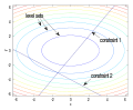  Level sets and constraint
• 
  Simple Lagrange multiplier example
• 
  Lagrange multiplier with one constraint
• 
  Basic Lagrange multiplier illustration
• 
  Lagrange_multiplier
• 
  Lagrange_multiplier